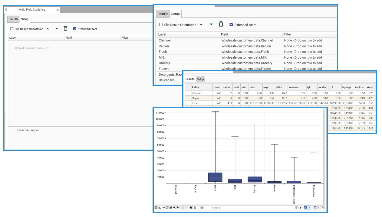
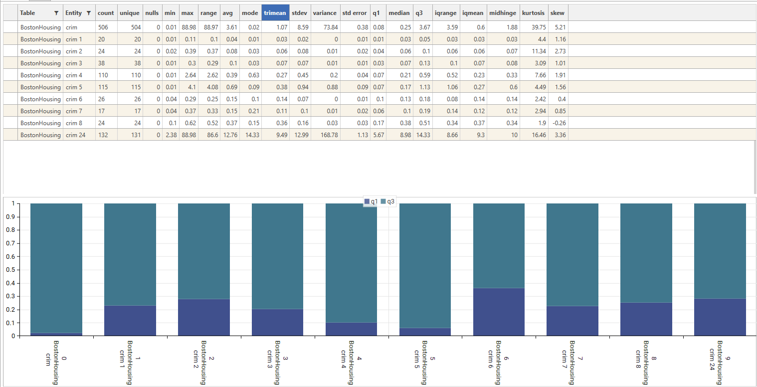
Multi-Field Statistics

Multi-Field Statistics allows statistics for multiple fields to be calculated and displayed in the same chart and/or grid.

It also supports the rapid creation of a dashboard of multiple individual statistics slots from up to 12 fields.

Results from the Multi-Field Statistics report can be exported into a table, ready for further analysis and engineering.

Report Layout

Quick Tip:

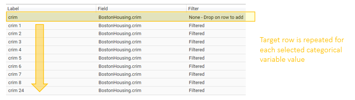
Drop a low cardinality field onto a measure and select Add Repeated Categorical Values from the popup menu to repeat the measure with a filter for each value.

Quick Tip:

Drop a table or field template onto the setup grid and select from:

Add All Discrete Numeric Fields - Adds all numeric fields in the table with datatype of discrete (up to 1024 fields)
Add All Numeric fields - Adds all numeric fields (up to 1024 fields)

Quick Tip:

Drop a filter on the result set to recalculate all fields with new dataset applied:

Report Setup

Adding Fields and filters

Fields

Add fields to the calculation by dragging and dropping from the Project Explorer. Drop onto the field list area: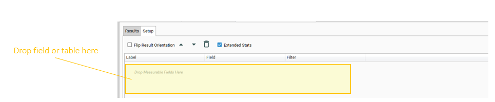

Drag the following object types:

Field(s) - add any field type -
- most statistics will only be calculated for numeric fields, and some will only be calculated for discrete numeric fields.
- drop a field onto a field already in the list and the helper menu will be displayed
Table- choose one of the following:
- Add all Discrete Field numeric fields
- Add all numeric fields
Field Template
- Drop an existing field template into the field list area and choose "Add All Fields"

Note!

All fields must come from the same table

Filters

Each row that is added to the field list can have a separate filter applied to it. To apply a filter to a row, drop the dataset onto the row in the field list. Select a row to see the filter details.

To apply a filter to the entire calcualtion, first calculate without the filter, and then drop the dataset onto the results grid.

Helper Menu

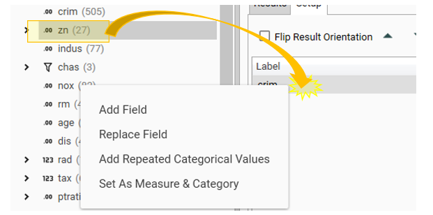
Add Field

Adds selected field to the list

Replace Field

Replaces the target field with the new field

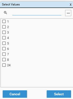
Add Repeated Categorical Values

Displays the "Select Values" dialog. Select the values to apply as filters. A row will be added for each value selected. Use the [...] help to control selection of values.

Set as Measure & Category

{TODO - What does this do?}

Select Fields

Hold CTRL or SHIFT keys to select multiple fields.

Re-arrange Fields

Use the arrow keys to move fields up and down in the calculation order

Remove Fields

Select the trashcan or right click and choose "Delete" to remove (a) field(s) from the calculation.

Create Template

Create a field template from selected fields by right-clicking and choosing "Create Template"

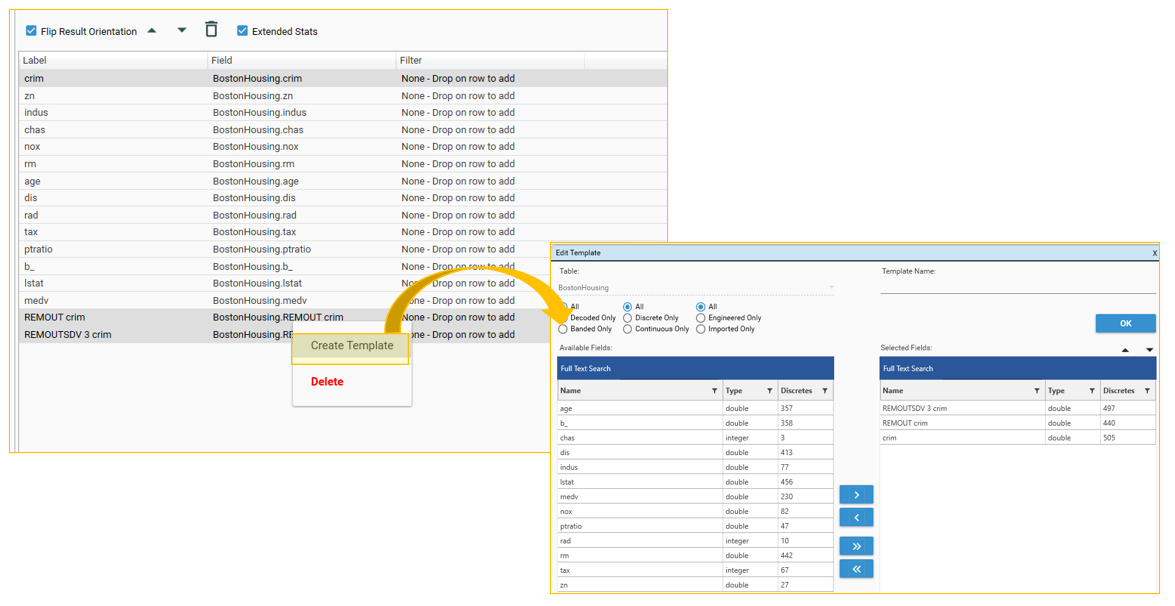
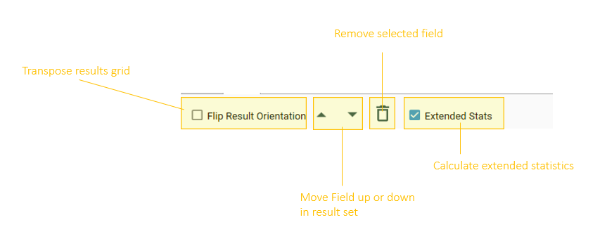
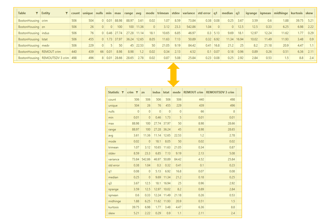
Transpose Results

Flip the orientation of the grid to have field names as either columns or rows.

Extended Stats

Calculate Extended statistics - on by default. (Note - Extended statistics are only calculated for numeric fields)

Available extended statistics (see Available Statistics for more details):

range
trimean
q1
q2 (median)
q3
iqmean
igrange
midhinge
kurtosis
skew

Calculate

There is no auto-calc on the multi-field statistics report. Once setup is complete, select the calculate button:

The result tab will automatically be displayed once the calculation is complete.

Results

Once the results tab is displayed, explore results further via the following options:

Right-Click

Right click a row in the grid and a helper menu will be displayed:

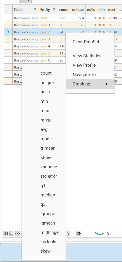
Clear Data Set - removes the base dataset if one is present. To check whether a dataset has been applied, open the info panel.
-----
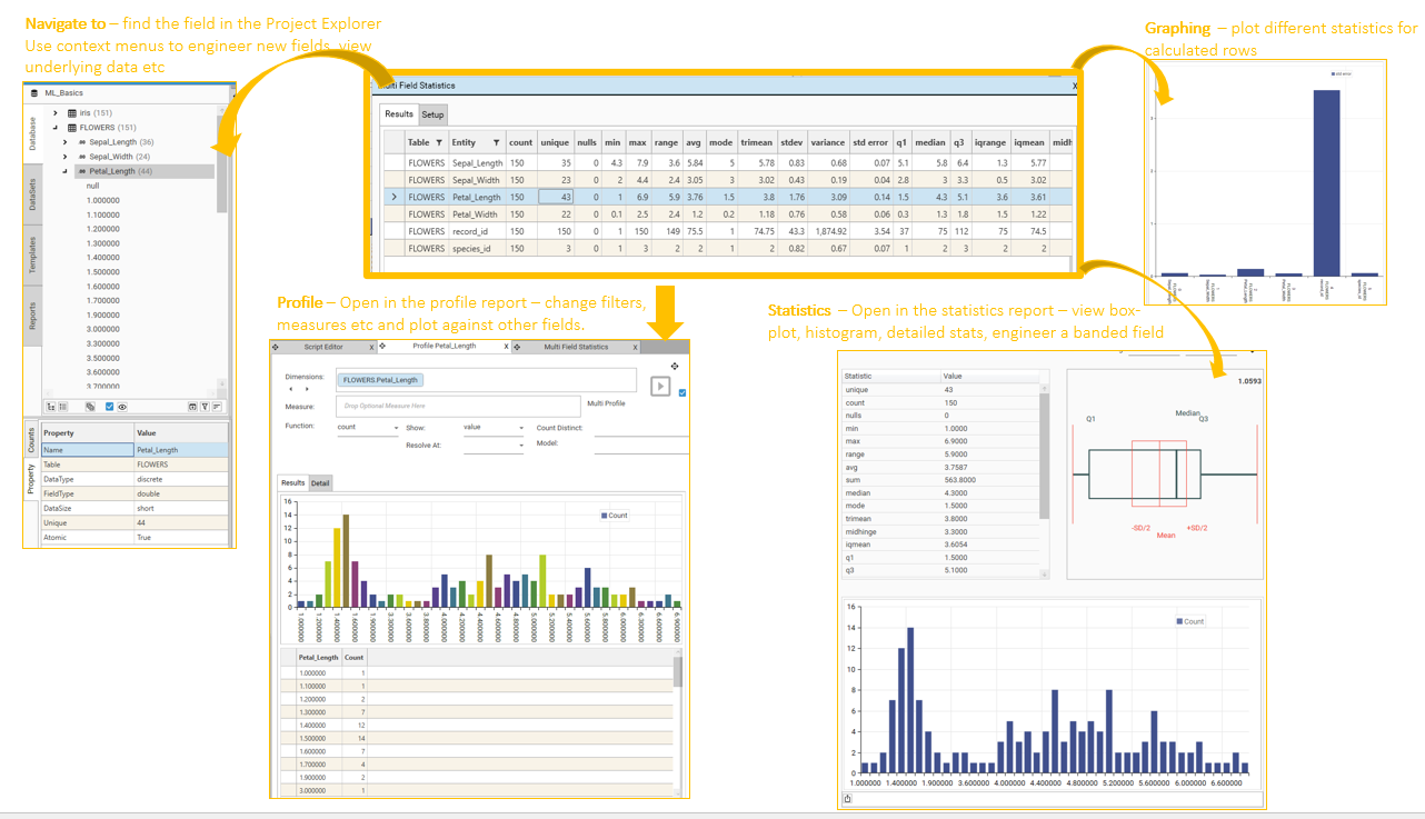
View Statistics - Opens the statistics report for the selected row. If a filter has been applied, it will be included in the report. Use the statistics report to see the detailed statistics, box-plot and histogram for the selected row. The statistics report can also be used to create a new banding or grouping from the field.
View Profile - Open the profile report for the selected row.
Navigate To - Open the selected field in Project Explorer. From here, view underlying data, create profiles, and engineer data.

Filter

Recalculate all statistics for a sub set of data by dropping a dataset onto the result grid.

Sort and Filter Results

The existing result set can be sorted and results from the results excluded or included by modifying column filters.

To sort: Click on a column header
To Filter: Select the table or field name to filter on

Controlling Display Options

See Micro Toolbar for details of the following:

Display options
- Grid only
- Chart only
- Grid and Chart
Sort Mode
Relative Width/Height
Grid/Chart display orientation
Export options

Box Plots

By default a box plot of all rows will be displayed. However, if specific statistics are being plotted via the graphing menu, a different kind of plot may be displayed. To return to a box-plot, select "Featured Report" from the charting option dropdown.

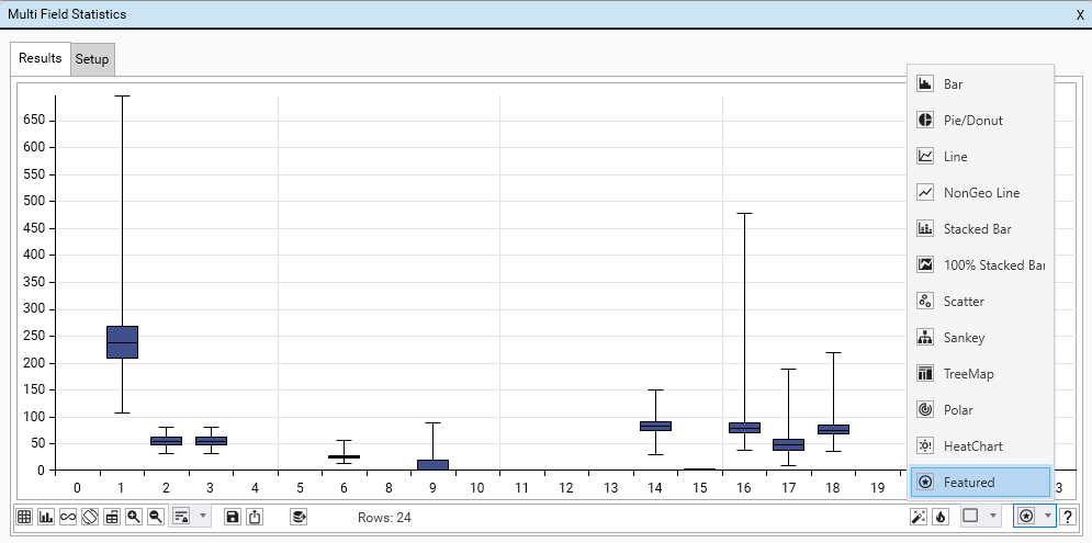
Visualisation

Visualisation can be controlled:

Via the usual charting and display options (see Micro-toolbar)
As part of setup.
By the right-click | Graphing option.

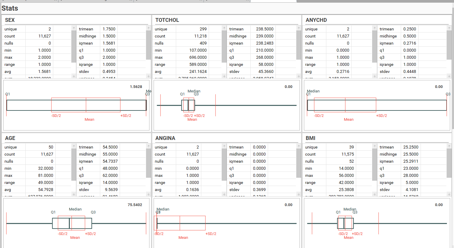
Create Dashboard

Automatically create a dashboard showing individual statistics for the first 12 rows in the result grid by choosing Automation (Open as Dashboard) from the micro-toolbar. To inspect a single variable in more detail, select the desired slot and choose "Open Copy"

Available Statistics

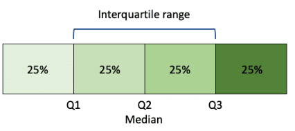
(The exclusive method is used to calculate the Interquartile range)

Statistic	Description	Calculation	Notes
avg	Mean The arithmetic mean value for the field in the Dataset	Sum of Values / Count of Values μ = (Σxᵢ) / N Where: μ (mu) is the population mean Σ (sigma) represents the summation (adding up) xᵢ represents each individual value in the population N is the total number of individuals in the population	Core Stats Describes the central tendency of the entire group being studied and is calculated by summing all the values and dividing by the total number of individuals in the population.
count	The number of records (or observations for the field) in the DataSet (including null)	number of observations	Core Stats Basic level of summarization, often represented in frequency charts and visualisations
iqmean	Interquartile mean Average of all the data points that lie within the interquartile range (IQR)	(Sum of data points between Q1 and Q3) / (Number of data points between Q1 and Q3)	Extended Stats A robust measure of central tendency that calculates the average of the data points within the interquartile range, providing a more representative "typical" value when outliers are present. IQMean and mean are close: suggests data is relatively symmetrical without significant outliers. IQMean noticeably different from mean: indicates data is likely skewed or has outliers IQMean and median are close: suggests middle 50% of data is relatively symmetrical. IQMean different from median: indicates middle 50% of data is not perfectly symmetrical. IQMean and trimean are similar: suggests relatively consistent distribution within the IQR
iqrange	IQR Represents the spread of the middle 50% of the data	IQR = Q3 – Q1	Extended Stats A robust measure of dispersion. Less sensitive to extreme values (outliers) than the range or standard deviation. This is because it focuses on the middle 50% of the data and ignores the values in the tails.
kurtosis	Describes the shape of the probability distribution. A measure of how "peaked" or "flat" the distribution is.		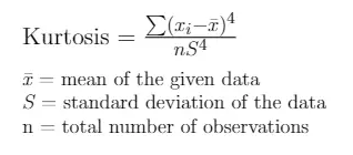Extended Stats Kurtosis indicates the "tailedness" of the distribution (i.e., how often outliers occur) ~3 : normal distribution >3 : fat tails (leptokurtic) <3 : thin tails (platykurtic) High Kurtosis (Leptokurtic): Indicates a higher probability of extreme values and a sharper peak. This might suggest a greater risk or volatility in the data. Low Kurtosis (Platykurtic): Indicates a lower probability of extreme values and a flatter peak. This might suggest a more stable or predictable dataset. Kurtosis near 3 (Mesokurtic): Suggests the distribution is similar in shape to a normal distribution.
max	The maximum value for the field in the Dataset	maximum value	Core Stats The highest value in the dataset
midhinge	Mid-Quartile Range A measure of central tendency that is less sensitive to extreme values (outliers) than the mean	(Q1 + Q3) / 2	Extended Stats Represents the centre of the Middle 50%: The midhinge represents the midpoint of the interquartile range (IQR). The IQR is the range between Q1 and Q3, encompassing the middle 50% of the data. Therefore, the midhinge is the centre of that middle 50%.
min	The minimum value for the field in the Dataset	minimum value	Core Stats The lowest value in the dataset
mode	The most commonly occurring value	Count occurrence of each value and select most commonly occurring value	Core Stats A measure of central tendency that represents the value or values that appear most frequently in a dataset. The mode is the most appropriate measure of central tendency for categorical data.
nulls	The number of null or empty records/observations		Core Stats The number of records with no observations
q1	First quartile. The 25th percentile. Lower quartile.	Arrange data in ascending order position = (n+1) * 0.25	Extended Stats Represented on a box plot as the lower edge of the box
q2 (median)	Middle value of the Dataset	Arrange data in ascending order position = (n+1)/2	Extended Stats Middle number in an ordered dataset. 50% of the data is below this value, 50% above.
q3	Third quartile. Upper Quartile. Middle value of second half of Dataset	Arrange data in ascending order position = (n+1) * 0.75	Extended Stats The value that separates lowest 75% of the data from highest 25% Represented on a box plot as the upper edge of the box
range	the total spread of values for the distribution	max - min	Extended Stats A simple measure of dispersion. Sensitive to outliers.
skew	skewness	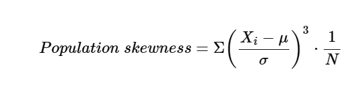Where: σ = population standard deviation X = data point µ = population mean N = population count	Extended Stats Skewness provides a measure of the "asymmetry" of a distribution. no skew (= 0) : mean = median right (+ve) skew (tail on the right) : mode < median < mean left (-ve) skew (tail on the left ) : mean < median
stdev	The standard deviation from the mean for all values in dataset	(Square root of variance) Square Root of [(Sum of square of differences from mean) / (number of data points -1) ] 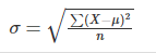Where: σ = population standard deviation X = data point µ = population mean n = population count	Core Stats Measures dispersion.
standard error	Estimate of variability of the calculated mean from the true population mean.	σx = standard deviation N = total number of observations	Core Stats A measure of how accurately the mean represents the true mean of the population.
sum	Total of all non-null values in the dataset	Sum of all values	Core Stats
trimean	A measure of central tendency - i.e., a representation of the "centre" of the data that gives the median twice the weight of the other quartiles	(Q1 + 2 * Q2 + Q3) / 4	Extended Stats Weighted average of the first quartile (Q1), the median (Q2), and the third quartile (Q3), giving more weight to the median. If trimean and mean are close, data is likely to be relatively symmetrical. If trimean noticeable different from mean, data is likely skewed or has outliers.
variance	Population variance	[(Sum of square of differences from mean) / (number of data points) ]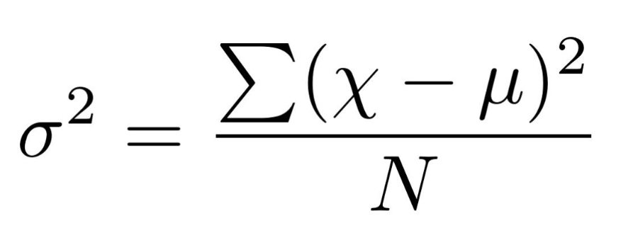 Where: σ = population standard deviation X = data point µ = population mean N = population count	Core Stats Variance is an indication of the "dispersion" of the data from the mean